5. Welding Example #02: TCP movements and Weaving#
In this example we will focus on more complex tcp movements along the workpiece and how to combine different motion shapes like weaving.
5.1. Imports#
# enable interactive plots on Jupyterlab with ipympl and jupyterlab-matplotlib installed
# %matplotlib widget
import numpy as np
import pandas as pd

from weldx import (
    Q_,
    CoordinateSystemManager,
    Geometry,
    LinearHorizontalTraceSegment,
    LocalCoordinateSystem,
    Trace,
    WXRotation,
    get_groove,
)
from weldx.welding.util import sine
5.2. General setup#
We will use the same workpiece geometry as defined in the previous example.
5.2.1. groove shape#
groove = get_groove(
    groove_type="VGroove",
    workpiece_thickness="0.5 cm",
    groove_angle="50 deg",
    root_face="1 mm",
    root_gap="1 mm",
)
5.2.2. workpiece geometry#
# define the weld seam length in mm
seam_length = Q_(150, "mm")

# create a linear trace segment a the complete weld seam trace
trace_segment = LinearHorizontalTraceSegment(seam_length)
trace = Trace(trace_segment)

# create 3d workpiece geometry from the groove profile and trace objects
geometry = Geometry(groove.to_profile(width_default=Q_(5, "mm")), trace)

# rasterize geometry
profile_raster_width = "2 mm"  # resolution of each profile in mm
trace_raster_width = "30 mm"  # space between profiles in mm
geometry_data_sp = geometry.rasterize(
    profile_raster_width=profile_raster_width, trace_raster_width=trace_raster_width
)
5.2.3. Coordinate system manager#
# crete a new coordinate system manager with default base coordinate system
csm = CoordinateSystemManager("base")

# add the workpiece coordinate system
csm.create_cs(
    coordinate_system_name="workpiece",
    reference_system_name="base",
    orientation=trace.coordinate_system.orientation.data,
    coordinates=Q_(trace.coordinate_system.coordinates.data, "mm"),
)

# add the geometry data of the specimen
csm.assign_data(
    geometry.spatial_data(profile_raster_width, trace_raster_width),
    "specimen",
    "workpiece",
)
5.3. Movement definitions#
Like in the previous example we start by defining the general linear movement along the weld seam with a constant welding speed.
tcp_start_point = Q_([5.0, 0.0, 2.0], "mm")
tcp_end_point = Q_([seam_length.m - 5.0, 0.0, 2.0], "mm")

v_weld = Q_(10, "mm/s")
s_weld = (tcp_end_point - tcp_start_point)[0]  # length of the weld
t_weld = s_weld / v_weld

t_start = pd.Timedelta("0s")
t_end = pd.Timedelta(str(t_weld))

rot = WXRotation.from_euler("x", 180, degrees=True)

coords = np.stack((tcp_start_point, tcp_end_point))

tcp_wire = LocalCoordinateSystem(
    coordinates=coords, orientation=rot, time=[t_start, t_end]
)
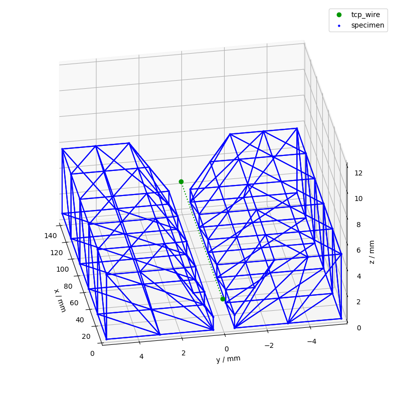
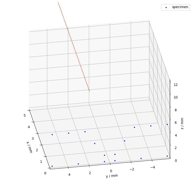
Let’s add the linear movement to the coordinate system manager and see a simple plot:
csm.add_cs(
    coordinate_system_name="tcp_wire", reference_system_name="workpiece", lcs=tcp_wire
)
csm

def ax_setup(ax, rotate=170):
    ax.legend()
    ax.set_xlabel("x / mm")
    ax.set_ylabel("y / mm")
    ax.set_zlabel("z / mm")
    ax.view_init(30, -10)
    ax.set_ylim([-5.5, 5.5])
    ax.view_init(30, rotate)
    ax.legend()


color_dict = {
    "tcp_sine": (255, 0, 0),
    "tcp_wire_sine": (255, 0, 0),
    "tcp_wire_sine2": (255, 0, 0),
    "tcp_wire": (0, 150, 0),
    "specimen": (0, 0, 255),
}
ax = csm.plot(
    coordinate_systems=["tcp_wire"],
    colors=color_dict,
    limits=[(0, 140), (-5, 5), (0, 12)],
    show_vectors=False,
    show_wireframe=True,
)
ax_setup(ax)
5.4. add a sine wave to the TCP movement#
We now want to add a weaving motion along the y-axis (horizontal plane) of our TCP motion. We can define a general weaving motion using the weldx.utility.sine function that creates TimeSeries class.
ts_sine = sine(f=Q_(0.5 * 2 * np.pi, "Hz"), amp=Q_([0, 0.75, 0], "mm"))
We now define a simple coordinate system that contains only the weaving motion.
tcp_sine = LocalCoordinateSystem(coordinates=ts_sine)
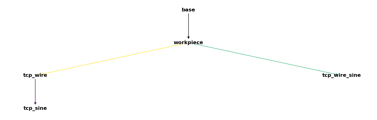
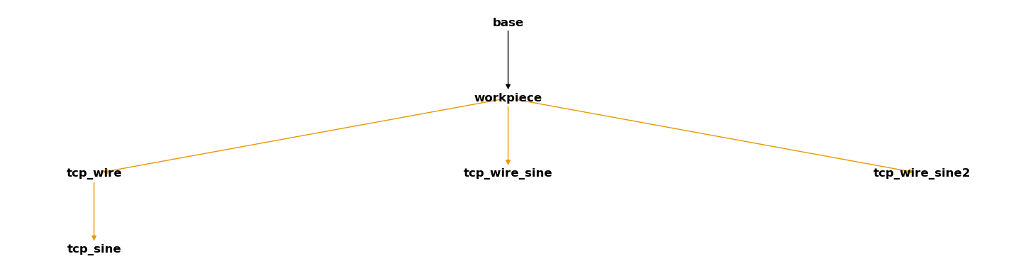
One approach to combine the weaving motion with the existing linear tcp_wire movement is to use the coordinate system manager. We can add the tcp_sine coordinate system relative to the tcp_wire system:
csm.add_cs(
    coordinate_system_name="tcp_sine", reference_system_name="tcp_wire", lcs=tcp_sine
)
csm

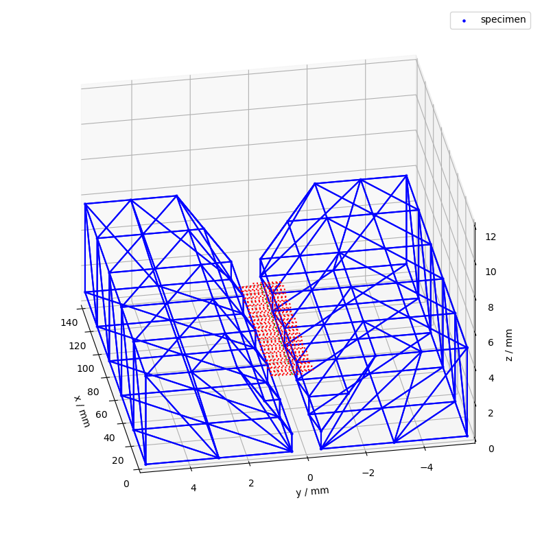
Lets see the result:
t = pd.timedelta_range(start=t_start, end=t_end, freq="10ms")
ax = csm.plot(
    coordinate_systems=["tcp_wire", "tcp_sine"],
    colors=color_dict,
    limits=[(0, 140), (-5, 5), (0, 12)],
    show_origins=False,
    show_vectors=False,
    show_wireframe=True,
    time=t,
)
ax_setup(ax)
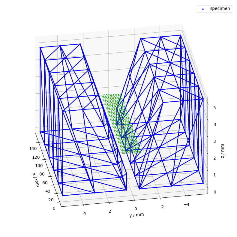
Here a little bit closer to see the actual sine wave:
ax = csm.plot(
    coordinate_systems=["tcp_wire", "tcp_sine"],
    colors=color_dict,
    limits=[(0, 5), (-2, 2), (0, 12)],
    show_origins=False,
    show_vectors=False,
    show_wireframe=False,
    time=t,
)
ax_setup(ax)
Another approach would be to combine both systems before adding them to the coordinate system manager. We can combine both coordinate systems using the + operator to generate the superimposed weaving coordinate system.
tcp_wire_sine = tcp_sine.interp_time(t) + tcp_wire
Note the difference in reference coordinate system compared to the first example.
csm.add_cs("tcp_wire_sine", "workpiece", tcp_wire_sine)
csm
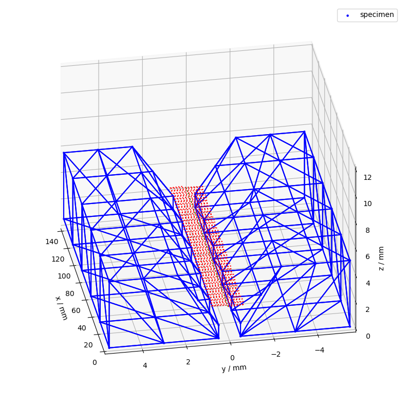
We get the same result:
ax = csm.plot(
    coordinate_systems=["tcp_wire", "tcp_wire_sine"],
    colors=color_dict,
    limits=[(0, 140), (-5, 5), (0, 12)],
    show_origins=False,
    show_vectors=False,
    show_wireframe=True,
)
ax_setup(ax)
ax = csm.plot(
    coordinate_systems=["tcp_wire", "tcp_sine"],
    colors=color_dict,
    limits=[(0, 5), (-2, 2), (0, 12)],
    show_origins=False,
    show_vectors=False,
    show_wireframe=False,
)
ax_setup(ax)
Adding every single superposition step in the coordinate system manager can be more flexible and explicit, but will clutter the CSM instance for complex movements.
5.5. plot with time interpolation#
Sometimes we might only be interested in a specific time range of the experiment or we want to change the time resolution. For this we can use the time interpolation methods of the CSM (or the coordinate systems).
Let’s say we want to weave only 8 seconds of our experiment (starting from 2020-04-20 10:03:00) but interpolate steps of 1 ms.
t_interp = pd.timedelta_range(start="3s", end="11s", freq="1ms")
ax = csm.interp_time(t_interp).plot(
    coordinate_systems=["tcp_wire", "tcp_wire_sine"],
    colors=color_dict,
    limits=[(0, 140), (-5, 5), (0, 12)],
    show_origins=False,
    show_vectors=False,
    show_wireframe=True,
)
ax_setup(ax)
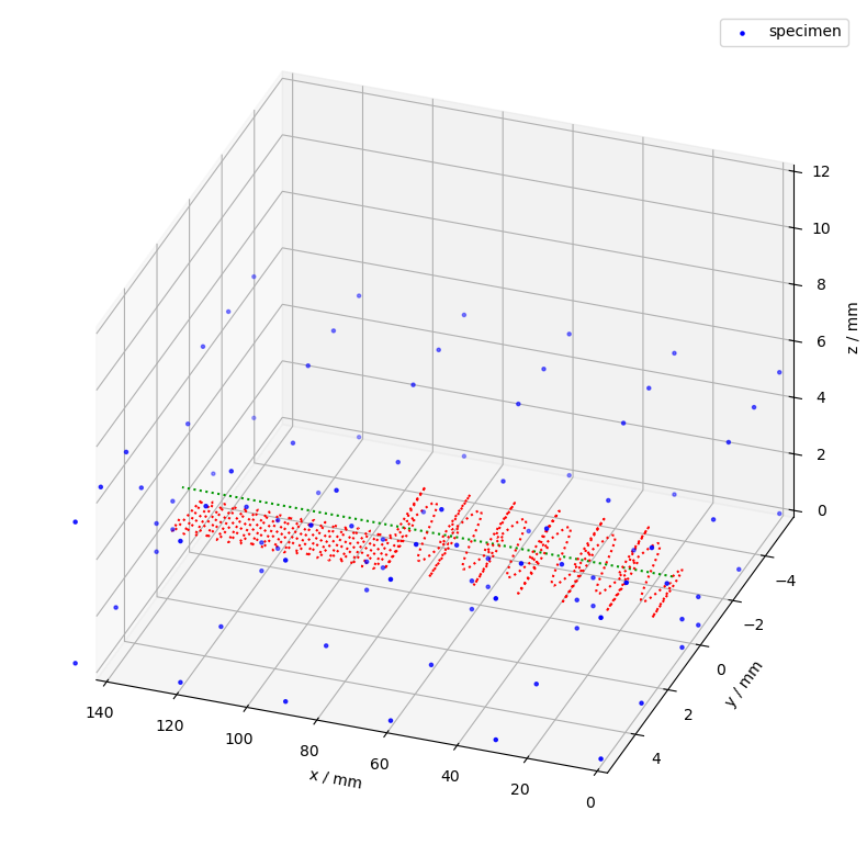
5.6. Adding a second weaving motion#
We now want to add a second weaving motion along the z-axis that only exists for a limited time. Lets generate the motion first:
ts_sine = sine(f=Q_(1 / 8 * 2 * np.pi, "Hz"), amp=Q_([0, 0, 1], "mm"))
We define a new LocalCoordinateSystem and interpolate it our specified timestamps.
t = pd.timedelta_range(start="0s", end="8s", freq="25ms")
tcp_sine2 = LocalCoordinateSystem(coordinates=ts_sine).interp_time(t)
tcp_sine2
<LocalCoordinateSystem> Size: 10kB
Dimensions:      (c: 3, v: 3, time: 321)
Coordinates:
  * c            (c) <U1 12B 'x' 'y' 'z'
  * v            (v) int64 24B 0 1 2
  * time         (time) timedelta64[ns] 3kB 00:00:00 ... 00:00:08
Data variables:
    orientation  (v, c) float64 72B 1.0 0.0 0.0 0.0 1.0 0.0 0.0 0.0 1.0
    coordinates  (time, c) float64 8kB [mm] 0.0 0.0 0.0 0.0 ... 0.0 0.0 0.9783
adding all the movements together. We have to be careful with the time-axis in this case !
t_interp = pd.timedelta_range(
    start=tcp_wire.time.index[0], end=tcp_wire.time.index[-1], freq="20ms"
)
tcp_wire_sine2 = (
    tcp_sine2.interp_time(t_interp) + tcp_sine.interp_time(t_interp)
) + tcp_wire
csm.add_cs("tcp_wire_sine2", "workpiece", tcp_wire_sine2)
csm
ax = csm.plot(
    coordinate_systems=["tcp_wire", "tcp_wire_sine2"],
    colors=color_dict,
    limits=[(0, 140), (-5, 5), (0, 12)],
    show_origins=False,
    show_vectors=False,
)
ax_setup(ax, rotate=110)
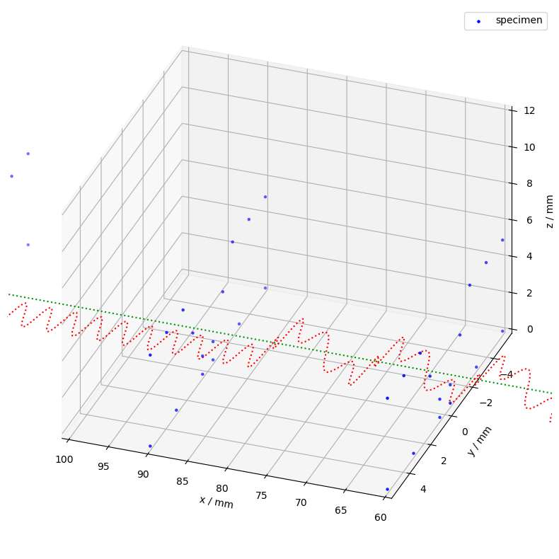
ax = csm.plot(
    coordinate_systems=["tcp_wire", "tcp_wire_sine2"],
    colors=color_dict,
    limits=[(60, 100), (-2, 2), (0, 12)],
    show_origins=False,
    show_vectors=False,
)
ax_setup(ax, rotate=110)
5.7. K3D Visualization#
csm.plot(
    backend="k3d",
    coordinate_systems=["tcp_wire_sine2"],
    colors=color_dict,
    show_vectors=False,
    show_traces=True,
    show_data_labels=False,
    show_labels=False,
    show_origins=True,
)