5. 3D Geometries

5.1. Introduction

In this tutorial we will describe how to create 3 dimensional structures that are based on one or more 2d profiles. We assume that you already know how to create 2d profiles using the weldx package. If this is not the case, please read the corresponding tutorial first.

You will learn:

• about the Trace class

• how to define a 3 dimensional geometry using the Geometry class

• how to specify geometries with varying cross sections using the VariableProfile class

Before we start, run the following code cells to include everything we need.

import matplotlib.pyplot as plt
from mpl_toolkits.mplot3d import Axes3D  # noqa: F401 unused import

import weldx.transformations as tf
from weldx import Q_
from weldx.geometry import (
    Geometry,
    LinearHorizontalTraceSegment,
    Profile,
    RadialHorizontalTraceSegment,
    Shape,
    Trace,
    VariableProfile,
    linear_profile_interpolation_sbs,
)
from weldx.transformations import LocalCoordinateSystem

5.2. Trace

The Trace class describes an arbitrary path through the 3 dimensional space. It is build from multiple segments that need to be passed to it when we create the Trace. Currently there are 2 segment types available: the LinearHorizontalTraceSegment that represents a straight line and the RadialHorizontalTraceSegment which describes a circular path. Both segment types have in common that the z-value remains constant and that they are free from torsion.

Let’s create one instance of each segment type. All you need to specify when creating a LinearHorizontalTraceSegment is its length:

line_segment = LinearHorizontalTraceSegment(length=Q_(10, "cm"))

That’s it. The RadialHorizontalTraceSegment needs a little bit more information. You need to provide its radius, rotation angle and if the rotation is clockwise or counter-clockwise:

arc_segment = RadialHorizontalTraceSegment(
    radius=Q_(15, "cm"), angle=Q_(90, "degree"), clockwise=True
)

Now that we have some segments, we can create a Trace. It expects a single segment or a list of segments as first argument. The individual segments get attached to each other in the same order as they are attached to the list. Each segment except for the first one gets its start orientation and coordinates from the end of the previous segment. The initial orientation and coordinates of the Trace can be provided in form of a LocalCoordinateSystem as optional second argument during the creation of the class instance. If you omit the second parameter, the Trace starts at the origin and is oriented in positive x-direction.

Here is an example:

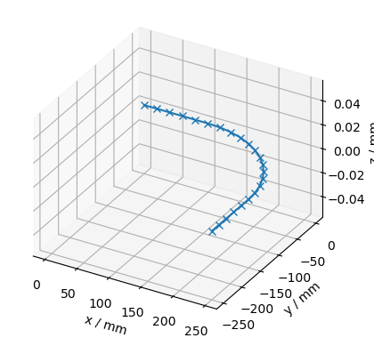
trace = Trace([line_segment, arc_segment, line_segment])

We can plot our Trace using the plot method:

trace.plot(raster_width=Q_(2, "cm"))

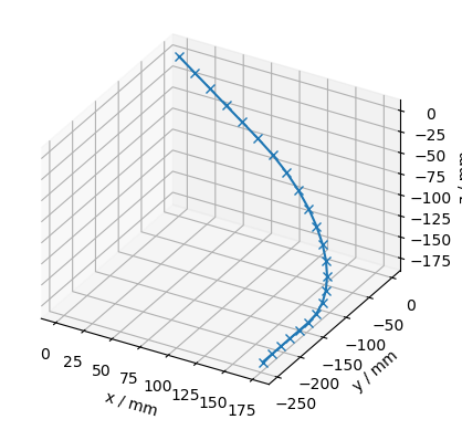
Let’s provide a initial coordinate system that is rotated by 45 degrees around the y-axis and see how that affects the result:

lcs_rot = LocalCoordinateSystem(
    tf.WXRotation.from_euler("y", Q_(45, "degree")).as_matrix()
)
trace_rot = Trace([line_segment, arc_segment, line_segment], lcs_rot)
trace_rot.plot(raster_width=Q_(2, "cm"))

Linear and radial trace segments already cover a lot of use cases but they are far from being enough to cover all possible needs. If you need more than those two basic segment types, there are two options. The first one is to implement your own segment type. This is discussed in detail in another tutorial.

TODO: Add link to tutorial once it is written

The second option, that you should prefer is the TODO: SOME_FANCY_NAME_SEGMENT. It enables you to describe the course of the trace segment with a mathematical function.

TODO: Continue once the segment type is implemented

5.3. Describing a 3d geometry

The simplest possible way to describe a 3 dimensional geometry using the weldx.geometry package is to create a 2d Profile and extrude it into 3d. The class that performs this action is called Geometry. It expects a Profile that defines the cross section as first argument and a Trace that describes the extrusion path as second one. Since we already have created a Trace all that is missing is a Profile. 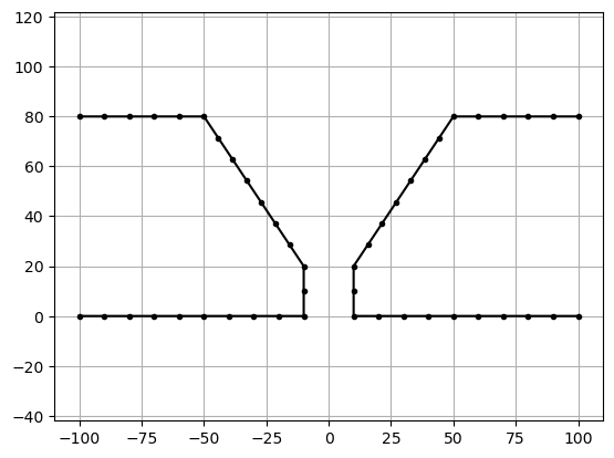So let’s create one:

shape_right = Shape().add_line_segments(
    Q_([[10, 8], [5, 8], [1, 2], [1, 0], [10, 0]], "cm")
)
shape_left = shape_right.reflect_across_line(Q_([0, 0], "cm"), Q_([0, 1], "cm"))
profile = Profile([shape_left, shape_right])
profile.plot(raster_width="1cm")

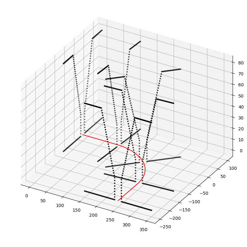
Now we can create and plot our Geometry:

geometry = Geometry(profile=profile, trace_or_length=trace)
geometry.plot(
    profile_raster_width=Q_(0.25, "cm"),
    trace_raster_width=Q_(10, "cm"),
    show_wireframe=False,
)
trace.plot(raster_width=Q_(1, "cm"), axes=plt.gca(), fmt="r-")

5.4. Geometries with varying cross section

The VariableProfile class gives us the opportunity to handle 3 dimensional geometries with a varying cross section. It can be used instead of a Profile during the creation of the Geometry class. Three pieces of information are necessary to create a VariableProfile.

First a list of profiles is required. This list represents “snapshots” of known cross sections along the extrusion path.

The second piece of information is a list of numbers that has the same number of elements as the list of profiles. Each of those numbers defines a coordinate on a 1 dimensional axis for the profile with the same list index. Their magnitude can be chosen arbitrarily with the exception that the first entry has to be 0 and the list items must be in ascending order. Due to the previously mentioned association between the coordinates/numbers and the profiles, the profiles are ordered by ascending coordinates. When you pass a VariableProfile to a Geometry, its first profile is used as the initial profile at the start of the Trace and the last as the one at the end. This relation enables the Geometry class to establish a linear coordinate transformation between the coordinates you specified in the VariableProfile and the corresponding position on the trace. For example, if you use three profiles with the coordinates [0, 25, 100] and your Trace has a length of $40 mm$, then the second profile occurs after $10 mm$ on the Trace.

The last thing we need to provide in order to create a VariableProfile is how the space between two profiles gets interpolated. We pass this information is form of a list that contains the corresponding interpolation functions. For each pair of profiles we need to specify an interpolation where the first list entry is associated with the first pair, the second entry with the second pair and so on. The number of list items is therefore one less than the number of profiles.

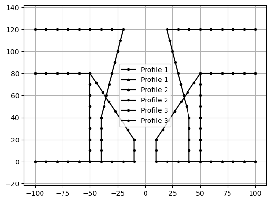
Lets have look at an example after this rather long text section. First, we define two more profiles.

shape_right_2 = Shape().add_line_segments(
    Q_([[10, 8], [5, 8], [5, 2], [5, 0], [10, 0]], "cm")
)
shape_left_2 = shape_right_2.reflect_across_line(Q_([0, 0], "cm"), Q_([0, 1], "cm"))
profile_2 = Profile([shape_left_2, shape_right_2])

shape_right_3 = Shape().add_line_segments(
    Q_([[10, 12], [2, 12], [4, 4], [4, 0], [10, 0]], "cm")
)
shape_left_3 = shape_right_3.reflect_across_line(Q_([0, 0], "cm"), Q_([0, 1], "cm"))
profile_3 = Profile([shape_left_3, shape_right_3])


profile.plot(raster_width=Q_(1, "cm"), label="Profile 1")
profile_2.plot(raster_width=Q_(1, "cm"), label="Profile 2", ax=plt.gca())
profile_3.plot(raster_width=Q_(1, "cm"), label="Profile 3", ax=plt.gca())
plt.gca().legend()

<matplotlib.legend.Legend at 0x7fda28fbeb50>

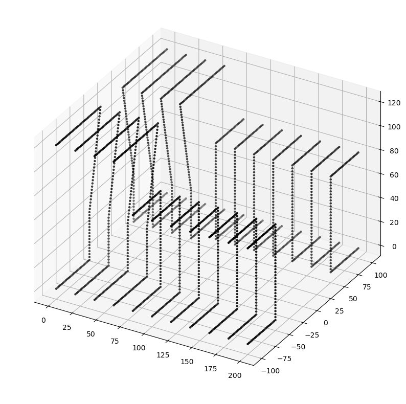
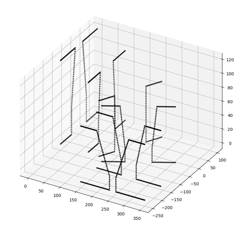
Now we create a VariableProfile, pass it to a new Geometry and plot it:

v_profile = VariableProfile(
    [profile_3, profile_2, profile],
    Q_([0, 40, 100], "cm"),
    [linear_profile_interpolation_sbs, linear_profile_interpolation_sbs],
)

geometry_vp = Geometry(profile=v_profile, trace_or_length=trace)
geometry_vp.plot(profile_raster_width=Q_(0.25, "cm"), trace_raster_width=Q_(8, "cm"))

<Axes3D: >

5.5. Custom interpolation schemes

You might notice that we used a interpolation function called linear_profile_interpolation_sbs. The “sbs” stands for “segment-by-segment”. It interpolates all of the profile segments linearly in the order as they appear in both involved profiles. So you need to assure that the segments are ordered accordingly in both profiles. It also requires that the number of segments is identical and it only works with the LineSegment.

You might wonder what alternative functions are provided, but currently there are none. The reason is that as soon as you start thinking about it, there are so many options that need to be considered that don’t have a unique solution that fits all use cases. To circumvent this issue, we provide the possibility to use custom interpolation functions. All that you need to do in order to use your own interpolation scheme is to define a python function with the following interface:

def custom_interpolation(Profile, Profile, float) -> Profile

The float parameter is a weighting factor representing the position on the trace segment between both profiles. The Geometry class will pass values between 0 and 1 where 0 is the beginning of the segment and associates with the first passed Profile. In conclusion, a value of 1 represents the end of the segment and is associated with the second Profile. What you do with this information is up to you. All that matters is that the function returns a valid Profile in the end.

Lets create an example interpolation that returns the first passed profile for weighting factors below 0.4 and the second one otherwise:

def my_interp(p0, p1, weight):
    if weight < 0.4:
        return p0
    return p1

Now we just create a VariableProfile with our new interpolation, combine it with a linear Trace inside of a Geometry and plot it:

v_profile_custom_interp = VariableProfile(
    [profile_3, profile_2], Q_([0, 1], "mm"), my_interp
)
trace_custom_interp = Trace(LinearHorizontalTraceSegment("20cm"))
geometry_custom_interp = Geometry(v_profile_custom_interp, trace_custom_interp)

geometry_custom_interp.plot(profile_raster_width="0.25cm", trace_raster_width="2cm")

<Axes3D: >