3. Welding groove types and definitions

3.1. Introduction

This tutorial is about generating different groove types and using the groove methods. The methods are seperatable in X parts:

• Creating a groove with get_groove

• Converting a groove to a profile

• Using plot on a profile constructed by a groove

• All possible groove types as plot

• Saving and loading grooves to/from weldx files

First starting with the imports needed for this tutorial:

from IPython.display import display

from weldx import WeldxFile, get_groove

3.2. Creating a groove

Each groove type has different input variables, which must be passed along with it. For this we need the Groove Type as string and the attributes that describe this Groove Type. All attributes are used with pint quantity, we recommend to use the quantity class created by us.

Here an Example with a V-Groove. Note that groove_type="VGroove" and the required attributes are workpiece_thickness, groove_angle, root_gap and root_face.

v_groove = get_groove(
    groove_type="VGroove",
    workpiece_thickness="1 cm",  # (note the use of 'cm')
    groove_angle="55 deg",
    root_gap="2 mm",
    root_face="1 mm",
)

display(v_groove)
print(str(v_groove))

VGroove(t=<Quantity(1, 'centimeter')>, alpha=<Quantity(55, 'degree')>, c=<Quantity(1, 'millimeter')>, b=<Quantity(2, 'millimeter')>, code_number=['1.3', '1.5'])

As shown above you pass the groove_type along with the attributes and get your Groove class. Function get_groove has a detailed description for all Groove Types and their Attributes.

Note: All classes can also be created separately with the classes, but this is not recommended.

from weldx.welding.groove.iso_9692_1 import VGroove

v_groove = VGroove(t, alpha, c, b)

3.3. Converting a groove to a profile

Each groove class can be converted into a Profile by calling its to_profile function. To learn more about the Profile class and its uses look into geometry_01_profiles.ipynb. Profiles created this way consist of one shape per mating part. For the V-Groove each mating part is made up of four basic lines.

v_profile = v_groove.to_profile()
print(v_profile)

Profile with 2 shape(s)
Shape 0:
Line: [-7.69 0.00] millimeter -> [-1.00 0.00] millimeter
Line: [-1.00 0.00] millimeter -> [-1.00 1.00] millimeter
Line: [-1.00 1.00] millimeter -> [-5.69 10.00] millimeter
Line: [-5.69 10.00] millimeter -> [-7.69 10.00] millimeter

Shape 1:
Line: [7.69 0.00] millimeter -> [1.00 0.00] millimeter
Line: [1.00 0.00] millimeter -> [1.00 1.00] millimeter
Line: [1.00 1.00] millimeter -> [5.69 10.00] millimeter
Line: [5.69 10.00] millimeter -> [7.69 10.00] millimeter

3.3.1. calculating groove cross sectional area

An approximation of the groove cross sectional area can be calculated via the cross_sect_area property

print(v_groove.cross_sect_area)

62.165931094691445 mm ** 2

3.4. Using plot on a profile constructed by a groove

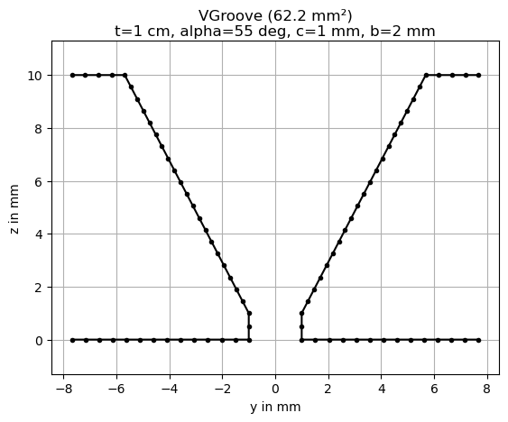
We can visualize the profile by simply calling the plot() function of the groove object. Carefully note the labeling (yz) and orientation of the axis. The plot shows the groove as seen along the negative x-axis (against the welding direction).

v_groove.plot()

As explained above you see that this V-groove has two halves and a V-Groove layout. The plot scaling is always in millimeter.

The plot method has the following attributes:

• title

  Setting from matplotlib. Default: None

• raster_width

  Is the ratio of the rasterized points between each joint.

• axis

  Setting from matplotlib. Default: equal

• grid

  Setting from matplotlib. Default: True

• line_style

  Setting from matplotlib. Default: '.'

• ax

  Setting from matplotlib. Default: None

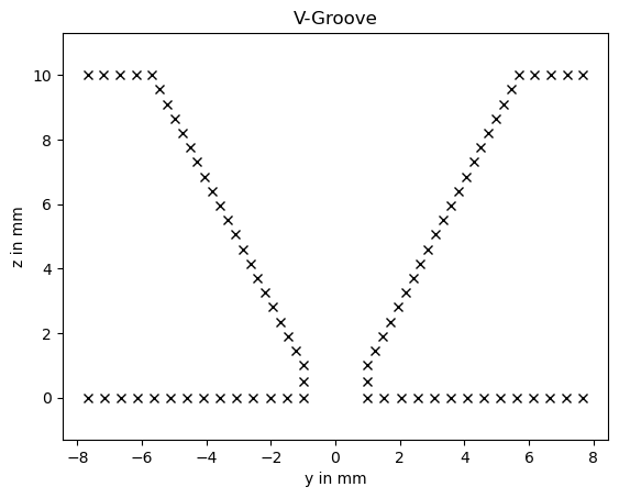
Here is the same plot with different options:

v_profile.plot(title="V-Groove", raster_width="0.5mm", grid=False, line_style="rx")

/home/docs/checkouts/readthedocs.org/user_builds/weldx/conda/latest/lib/python3.9/site-packages/weldx/geometry.py:1457: UserWarning: color is redundantly defined by the 'color' keyword argument and the fmt string "rx" (-> color='r'). The keyword argument will take precedence.
  ax.plot(segment[0], segment[1], line_style, label=label, color=c)

3.5. using ASDF

All groove types can be saved to weldx-files.

Here we demonstrate the writing of the groove data into a buffer (in-memory file):

tree = dict(test_v_groove=v_groove)
file = WeldxFile(tree=tree, mode="rw")

We can show the file header with all groove metadata:

file.header()

#ASDF 1.0.0
#ASDF_STANDARD 1.5.0
%YAML 1.1
%TAG ! tag:stsci.edu:asdf/
%TAG !weldx! asdf://weldx.bam.de/weldx/tags/
--- !core/asdf-1.1.0
asdf_library: !core/software-1.0.0 {author: The ASDF Developers, homepage: 'http://github.com/asdf-format/asdf',
  name: asdf, version: 2.15.0}
history:
  extensions:
  - !core/extension_metadata-1.0.0
    extension_class: asdf.extension.BuiltinExtension
    software: !core/software-1.0.0 {name: asdf, version: 2.15.0}
  - !core/extension_metadata-1.0.0
    extension_class: weldx.asdf.extension.WeldxExtension
    extension_uri: asdf://weldx.bam.de/weldx/extensions/weldx-0.1.2
    software: !core/software-1.0.0 {name: weldx, version: 0.6.7.dev4+g5429056.d20230521}
test_v_groove: !weldx!groove/iso_9692_1_2013_12/VGroove-0.1.0
  t: !weldx!units/quantity-0.1.0 {value: 1, units: !weldx!units/units-0.1.0 centimeter}
  alpha: !weldx!units/quantity-0.1.0 {value: 55, units: !weldx!units/units-0.1.0 degree}
  b: !weldx!units/quantity-0.1.0 {value: 2, units: !weldx!units/units-0.1.0 millimeter}
  c: !weldx!units/quantity-0.1.0 {value: 1, units: !weldx!units/units-0.1.0 millimeter}
  code_number: ['1.3', '1.5']

Now we are taking a copy of the first file by calling WeldxFile.write_to. Then we read the file contents again and validating the extracted groove:

file_copy = file.write_to()
data = WeldxFile(file_copy)
data["test_v_groove"]

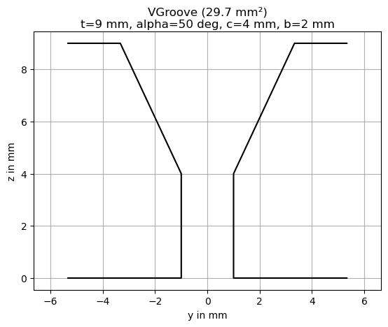
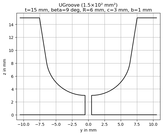
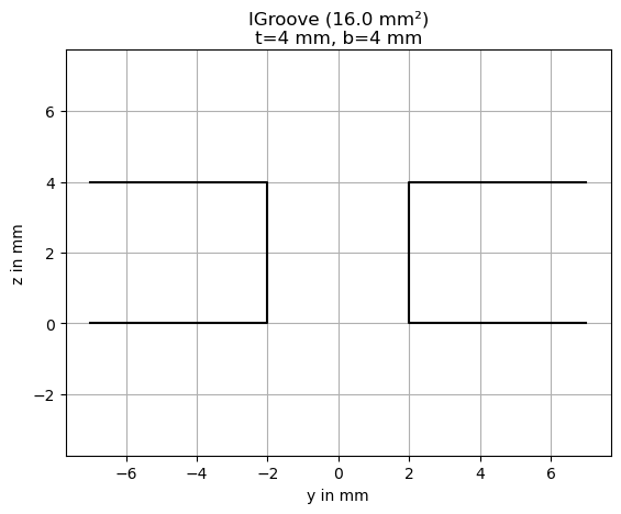
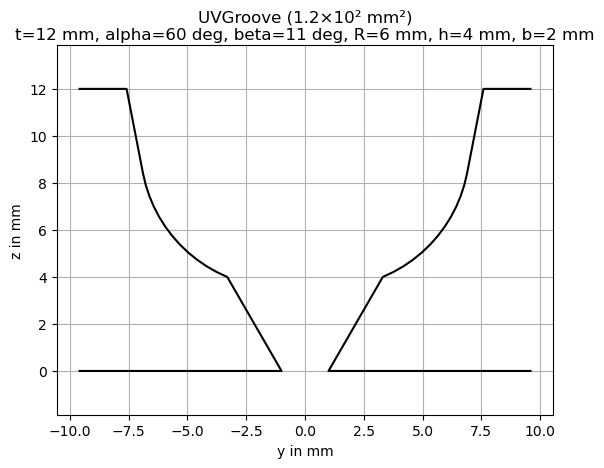
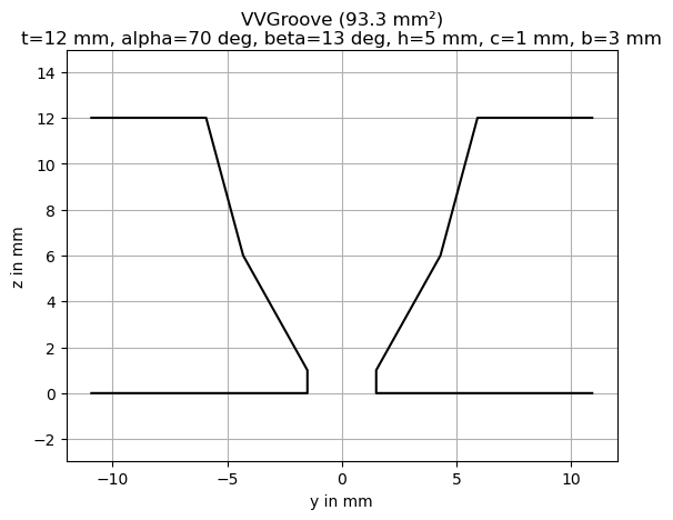
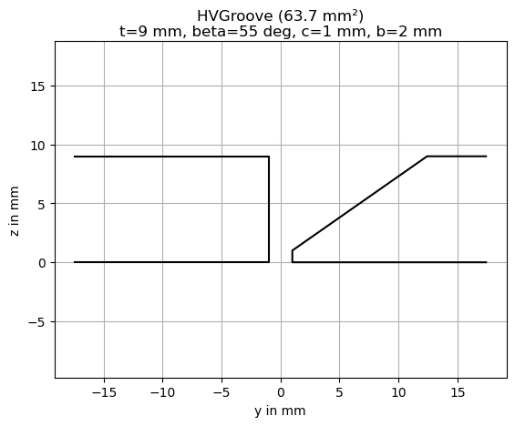
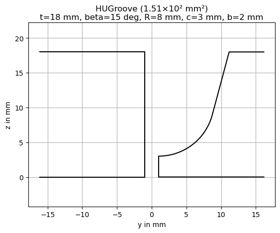
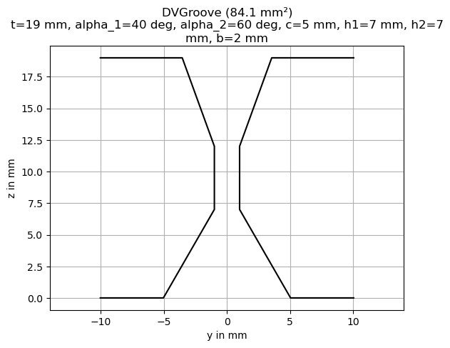
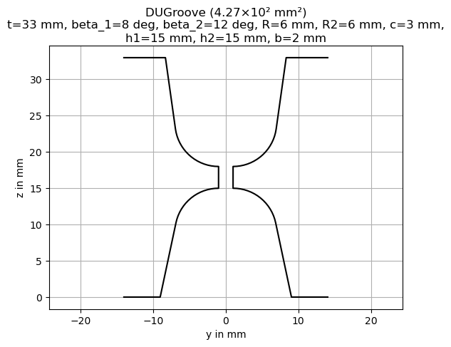
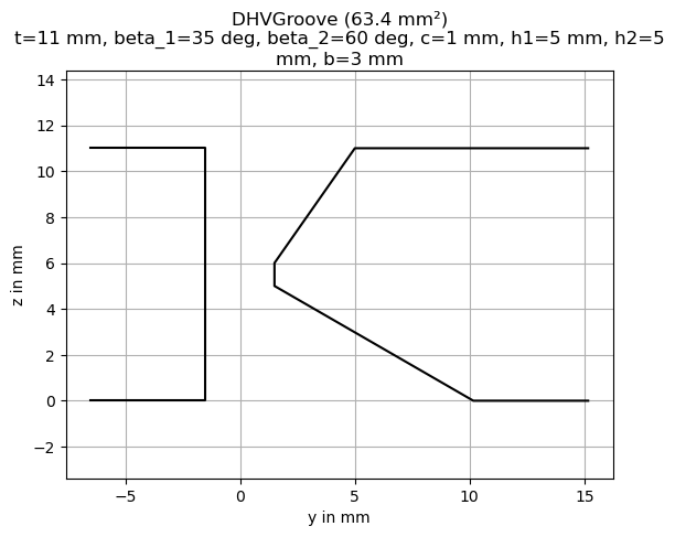
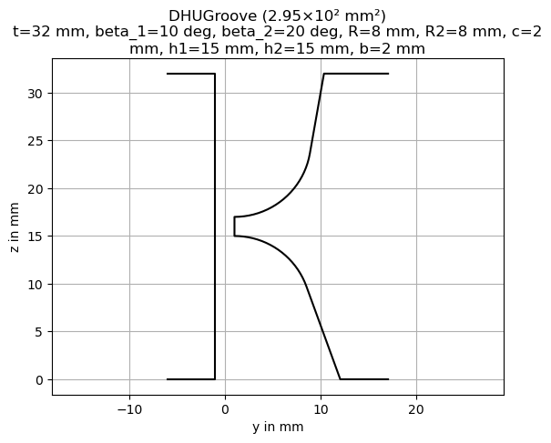
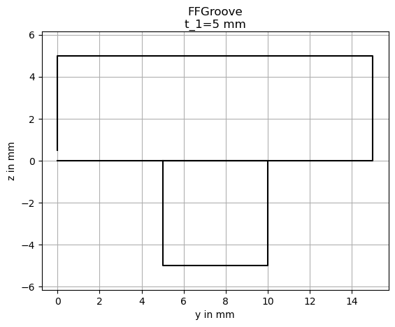
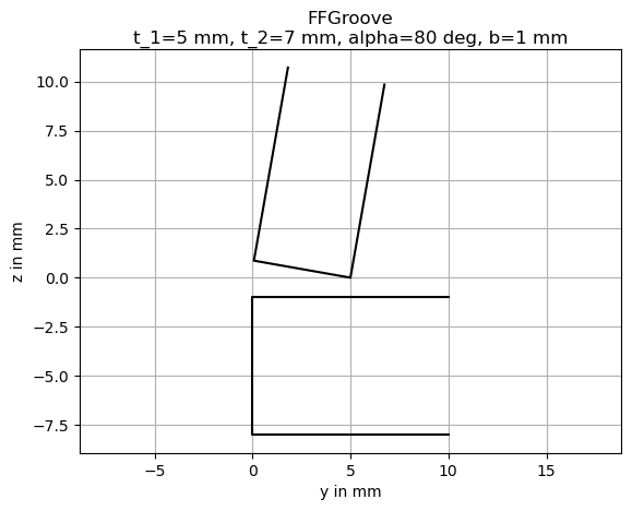
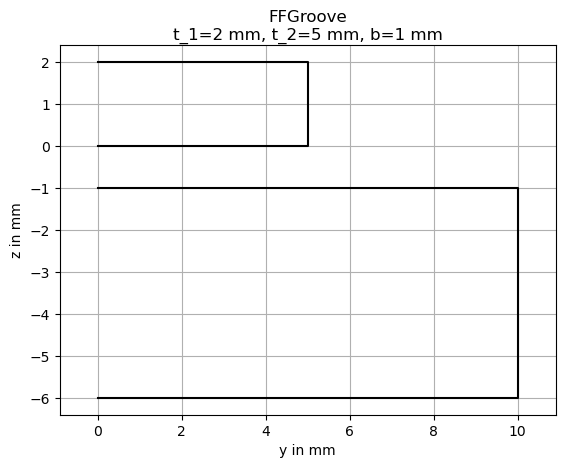
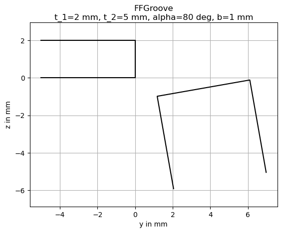
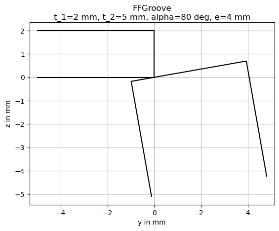
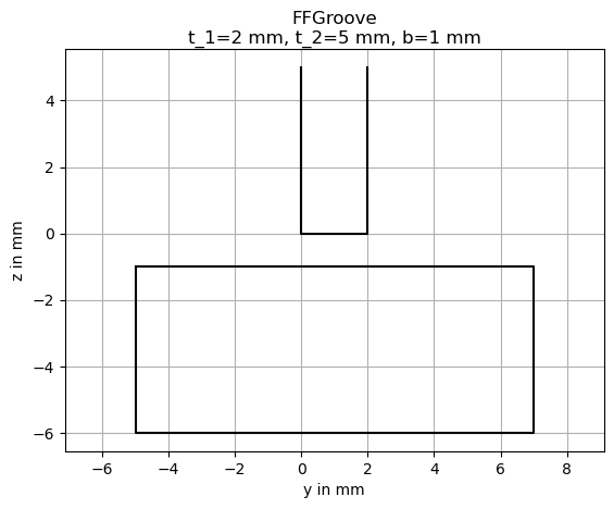
3.6. Examples of all possible Groove Types

An overview of all possible groove types:

# generate test grooves
from weldx.welding.groove.iso_9692_1 import _create_test_grooves

groove_dict = _create_test_grooves()
for k in ["dv_groove2", "dv_groove3", "du_groove2", "du_groove3", "du_groove4"]:
    groove_dict.pop(k, None)

for _k, v in groove_dict.items():
    v[0].plot(line_style="-")