1. Transformations Tutorial #1: Coordinate Systems

1.1. Introduction

This tutorial is about the transformation packages LocalCoordinateSystem class which describes the orientation and position of a Cartesian coordinate system towards another reference coordinate system. The reference coordinate systems origin is always at $(0, 0, 0)$ and its orientation is described by the basis: $e_x = (1, 0, 0)$, $e_y = (0, 1, 0)$, $e_z = (0, 0, 1)$. All coordinate systems used by WelDX are positively oriented and follow the right hand rule.

Note that this tutorial contains some chapters that address low-level features that will be seldom required when working with WelDX because there are better alternatives. The purpose of those chapters is mainly to give a complete overview over the capabilities of the LocalCoordinateSystem class. We will inform you at the beginning of a chapter if you can skip it without missing out on some important information.

1.2. Imports

# enable interactive plots on Jupyterlab with ipympl and jupyterlab-matplotlib installed
# %matplotlib widget

# interactive plots
import numpy as np
import pandas as pd
import xarray as xr

import weldx.visualization as vs
from weldx import Q_, LocalCoordinateSystem, MathematicalExpression, TimeSeries

1.3. Construction

The initializer of the LocalCoordinateSystem class takes 2 parameters, the orientation and the coordinates. orientation requires a 3x3 matrix. It can either be viewed as a rotation/reflection matrix or a set of normalized column vectors that represent the 3 basis vectors of the coordinate system inside of the reference system. The matrix needs to be orthogonal, otherwise, an exception is raised. coordinates is the position of the LocalCoordinateSystem’s origin inside the reference coordinate system. The default parameters are the identity matrix and the zero vector. Hence, we get a system that is identical to the reference system if no parameter is passed to the constructor:

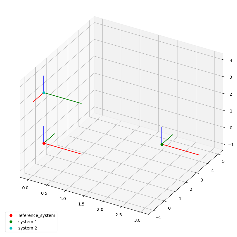
lcs_ref = LocalCoordinateSystem()

We now create some additional coordinate systems. Note that coordinates can not be provided as pure numbers but need to be quantities. This ensures that coordinates always have a unit. If quantities are new to you, checkout the documentation of the pint package.

lcs_01 = LocalCoordinateSystem(coordinates=Q_([2, 4, -1], "mm"))

rotation = [[0, 1, 0], [-1, 0, 0], [0, 0, 1]]
lcs_02 = LocalCoordinateSystem(orientation=rotation, coordinates=Q_([0, 0, 3], "mm"))

lcs_01 has the same orientation as the reference system but a different position. lcs_02 also risides at a position different from the origin. Additionally, it is rotated around the z-axis by 90 degrees. Below, a plot of the 3 coordinate systems is shown.

Note that the corresponding code cell that produces the plot might be hidden since its content is not relevant for this tutorial. This is also the case for all further plots. If those cells are not hidden, just ignore the code and focus on the plots.

HINT: Enabled interactive plots in the jupyter notebook version of this tutorial by uncommenting the code in the first cell. If you do so, you can rotate the plot by pressing the left mouse button and moving the mouse. This helps to understand how the different coordinate systems are positioned in the 3d space.

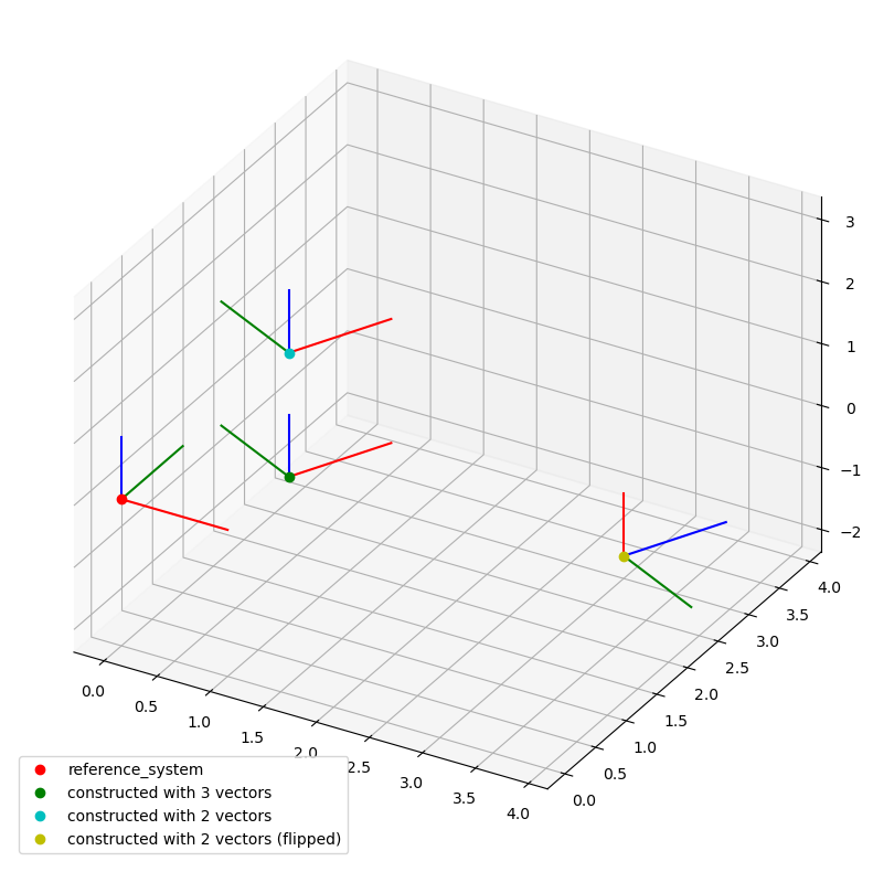
Since writing down a rotation matrix is usually not as straight forward as a translation vector, there are some additional methods to create a LocalCoordinateSystem that let you describe the systems orientation in a more intuitive way. With the from_axis_vectors method, you specify orthogonal vectors that point into the same directions as the basis vectors of the new coordinate system. 2 vectors are usually sufficient since the third one can be computed automatically but you can also provide all three.

As an example take these 3 orthogonal vectors of arbitrary length:

a = [1, 2, 0]
b = [-6, 3, 0]
c = [0, 0, 5]

If they are orthogonal, we can use them to specify the orientation of a new LocalCoordinateSystem. So let’s try that:

lcs_03 = LocalCoordinateSystem.from_axis_vectors(
    x=a, y=b, z=c, coordinates=Q_([1, 1, 0], "mm")
)

Seems like it worked. If those vectors weren’t orthogoal, an exception would have been raised as the following example demonstrates:

w = [1, 0, 1]
try:
    LocalCoordinateSystem.from_axis_vectors(
        x=a, y=b, z=w, coordinates=Q_([1, 1, 0], "mm")
    )
except ValueError as e:
    print(f"The following exception was raised:\n{e}")

The following exception was raised:
Orientation vectors must be orthogonal

If we want the third vector to be calculated automatically, we pass just the two vectors we know:

lcs_04 = LocalCoordinateSystem.from_axis_vectors(
    x=a, z=c, coordinates=Q_([1, 1, 2], "mm")
)

Because we used the vectors from before, the orientations of both created coordinate systems should be identical. Let’s check that:

np.allclose(lcs_03.orientation, lcs_04.orientation)

True

Note that order matters here. If we flipped a and c as x- and z-axis, the calculated third axis would point into the opposite direction because WelDX always calculates the missing one in a way that the resulting system is positively oriented:

lcs_flipped_y = LocalCoordinateSystem.from_axis_vectors(
    x=c, z=a, coordinates=Q_([3, 3, -2], "mm")
)

Here is a plot of the created coordinate systems:

<Axes3D: >

Another method to create a LocalCoordinateSystem is from_euler. It utilizes a series of rotations around the reference systems’ coordinate axis to describe the new systems orientation. Its sequence parameter expects a string that determines the rotation sequence around the coordinate axes from left to right. For example, "xyz" expresses that the first rotation is around the x-axis, the second around the y-axis, and the last around the z-axis. angles is either a scalar for a single rotation or a list for a series of rotations. As the name suggests, it defines the rotation angles in the same order as the given sequence. The parameter degrees should be set to True if the provided angles are in degrees. 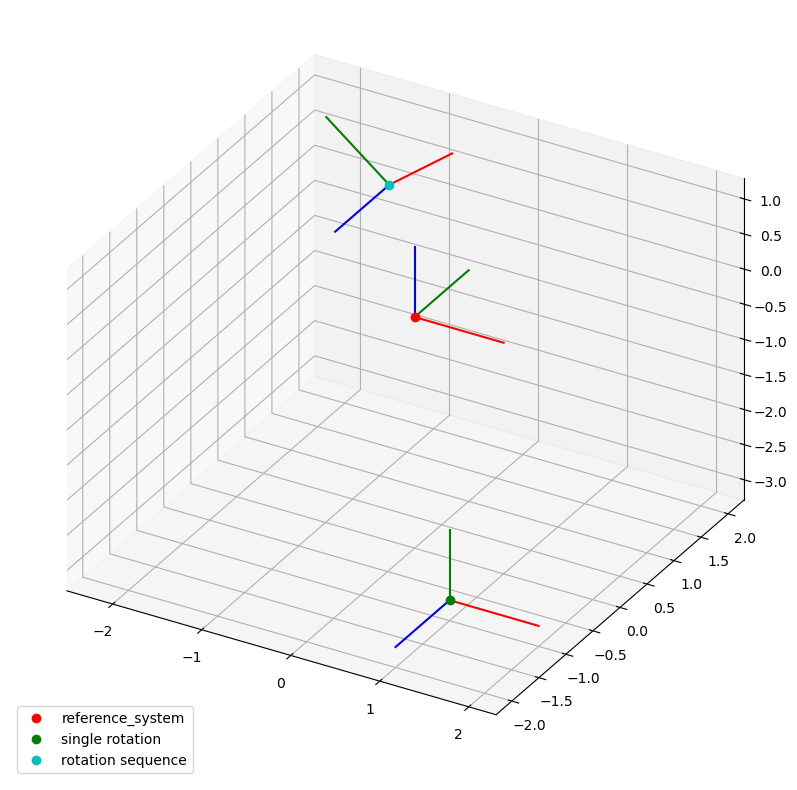Here is a short example for a single rotation:

lcs_05 = LocalCoordinateSystem.from_euler(
    sequence="x", angles=90, degrees=True, coordinates=Q_([1, -1, -3], "mm")
)

A rotation sequence would be defined as follows:

lcs_06 = LocalCoordinateSystem.from_euler(
    sequence="xy", angles=[90, -45], degrees=True, coordinates=Q_([-1.5, 2, 0], "mm")
)

The plot looks like this:

1.4. Coordinate transformations

Note: This chapter covers rather low-level details. Coordinate transformations in WelDX should generally be done using the CoordinateSystemManager class (click to open tutorial) since it is much easier to use and you do not need to remember some conventions mentioned below. You won’t have any problems in understanding WelDX if you skip this chapter entirely.

It is quite common that there exists a chain or tree-like dependency between coordinate systems. We might have a moving object with a local coordinate system that describes its position and orientation towards a fixed reference coordinate system. This object can have another object attached to it, with its position and orientation given in relation to its parent objects coordinate system. If we want to know the attached object coordinate system in relation to the reference coordinate system, we have to perform a coordinate transformation.

To avoid confusion about the reference systems of each coordinate system, we will use the following naming convention for the coordinate systems: lcs_NAME_in_REFERENCE. This is a coordinate system with the name “NAME” and its reference system has the name “REFERENCE”. The only exception to this convention will be the root coordinate system lcs_ref, which has no reference system.

The LocalCoordinateSystem class provides the + and - operators to change the reference system easily. The + operator will transform a coordinate system to the reference coordinate system of its current reference system:

lcs_child_in_ref = lcs_child_in_parent + lcs_parent_in_ref

As the naming of the variables already implies, the + operator should only be used if there exists a child-parent relation between the left-hand side and right-hand side system. If two coordinate systems share a common reference system, the - operator transforms one of those systems into the other:

lcs_child_in_parent = lcs_child_in_ref - lcs_parent_in_ref

It is important to remember that this operation is in general not commutative since it involves matrix multiplication which is also not commutative. During those operations, the local system that should be transformed into another coordinate system is always located to the left of the + or - operator. You can also chain multiple transformations, like this:

lcs_A_in_C = lcs_A_in_B + lcs_B_in_ref - lcs_C_in_ref

Pythons operator associativity (link) for the + and - operator ensures, that all operations are performed from left to right. So in the previously shown example, we first calculate an intermediate coordinate system lcs_A_in_ref (lcs_A_in_B + lcs_B_in_ref) without actually storing it to a variable and subsequently transform it to the reference coordinate system C (lcs_A_in_ref - lcs_C_in_ref). Keep in mind, that the intermediate results and the coordinate system on the right-hand side of the next operator must either have a child-parent relation (+ operator) or share a common coordinate system (- operator), otherwise the transformation chain produces invalid results.

You can think about both operators in the context of a tree-like graph structure where all dependency chains lead to a common root coordinate system. The + operator moves a coordinate system 1 level higher and closer to the root. Since its way to the root leads over its parent coordinate system, the parent is the only valid system than can be used on the right-hand side of the + operator. The - operator pushes a coordinate system one level lower and further away from the root. It can only be pushed one level deeper if there is another coordinate system connected to its parent system.

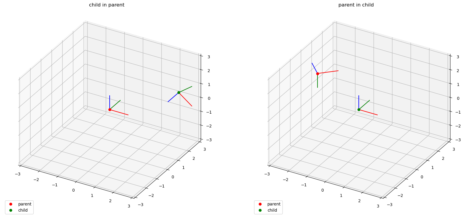
1.5. Invert method

The invert method calculates how a parent coordinate system is positioned and oriented in its child coordinate system:

lcs_child_in_parent = lcs_parent_in_child.invert()

Here is a short example with visualization:

lcs_child_in_parent = LocalCoordinateSystem.from_euler(
    sequence="xy", angles=[90, 45], degrees=True, coordinates=Q_([2, 3, 0], "mm")
)

lcs_parent_in_child = lcs_child_in_parent.invert()

1.6. Time dependency

The orientation and position of a LocalCoordinateSystem towards their reference system might vary in time. For example, in a welding process the position of the torch towards the specimen is changing constantly. The LocalCoordinateSystem provides an interface for such cases. All previously shown construction methods also provide the option to pass a time parameter.

To create a time-dependent system, you have to provide a list of time values. WelDX supports several time formats. A list of the supported formats can be found in the documentation of the generalized Time class.

If you use the time parameter, you also need to provide the extra data for the orientation and/or coordinates to the construction method. One way to do this is by providing an array of coordinate vectors or orientation matrices with the same number of elements as there are time values. For example: If you want to create a moving coordinate system with 2 timestamps, you can do it by like this:

time = ["2010-02-01", "2010-02-02"]

coordinates_mov = Q_([[-3, 0, 0], [0, 0, 2]], "mm")

lcs_mov_in_ref = LocalCoordinateSystem(coordinates=coordinates_mov, time=time)

Note that the coordinates are now a 2-dimensional array with two coordinate vectors while the orientation is still a single matrix (the default unit matrix) and therefore constant.

A coordinate system with varying orientation between 2 timestamps using the from_axis_vectors can be defined very similar:

x_vecs = [[1, 0, 0], [0, -1, 0]]
y_vecs = [[0, 1, 0], [1, 0, 0]]
coordinates_rot = Q_([1, 0, 2], "mm")

lcs_rot_in_ref = LocalCoordinateSystem.from_axis_vectors(
    x=x_vecs, y=y_vecs, coordinates=coordinates_rot, time=time
)

Here the individual vectors are arrays.

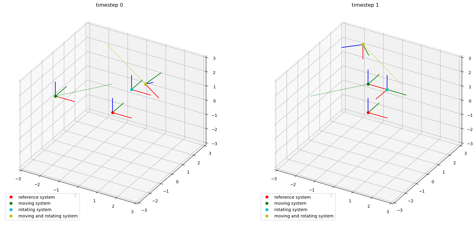
A rotating and moving coordinate system defined with the from_euler method is shown in the next code section:

angles = [[25, 45], [135, 90]]
coordinates_movrot = Q_([[0, 3, 0], [-2, 3, 2]], "mm")

lcs_movrot_in_ref = LocalCoordinateSystem.from_euler(
    sequence="xy",
    angles=angles,
    degrees=True,
    coordinates=coordinates_movrot,
    time=time,
)

Here is a visualization of the created coordinate systems at the two different times:

1.7. Time interpolation

It is also possible, to interpolate a coordinate system’s orientations and coordinates in time by using the interp_time function. You have to pass it a single or multiple target times for the interpolation. The same time formats that are compatible with the different construction methods can be used here too.

Alternatively, you can pass another LocalCoordinateSystem which provides the target timestamps. The return value of this function is a new LocalCoordinateSystem with interpolated orientations and coordinates. In case that a target time for the interpolation lies outside of the LocalCoordinateSystems’ time range, the boundary value is broadcasted.

Here is an example:

time = ["2010-02-02", "2010-02-07"]
time_interp = [
    "2010-02-01",
    "2010-02-03",
    "2010-02-04",
    "2010-02-05",
    "2010-02-06",
    "2010-02-11",
]

coordinates_tdp = Q_([[0, 3, 0], [-2, 3, 2]], "mm")
angles_tdp = [0, 90]

lcs_tdp_in_ref = LocalCoordinateSystem.from_euler(
    sequence="z",
    angles=angles_tdp,
    degrees=True,
    coordinates=coordinates_tdp,
    time=time,
)

lcs_interp_in_ref = lcs_tdp_in_ref.interp_time(time_interp)

Here is a visual representation of the original and the interpolated system:

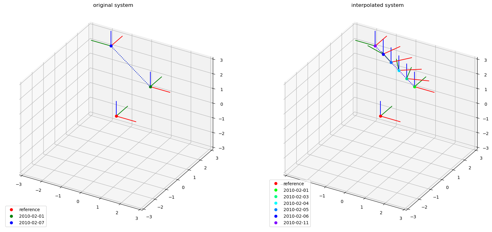
As you can see, the time values "2010-02-01" and "2010-02-11", which lie outside the original range from "2010-02-02" and "2010-02-07", still get valid values due to the broadcasting across time range boundaries. The intermediate coordinates and orientations are interpolated as expected.

Note: Using the + and - operators with time dependent systems obeys the following rules:

• If the left-hand side system has a time component, the data of the right-hand side system will be interpolated to the same times

• In case, that the left-hand side system has no time component, but the right-hand side does, the resulting system has the same time components as the right-hand side system

1.8. Mathematical Expressions for time dependent coordinates

Another type that can be used when creating a LocalCoordinateSystem is the TimeSeries. This class represents time-dependent data and can either be created with explicit values or a MathematicalExpression (click to get to API doc). Therefore, we can describe time dependent coordinate systems also with mathematical expressions (Note that only coordinates support the TimeSeries class at the moment).

We will give you just a short example without much explanation here, but if you want to learn how to create a valid TimeSeries using mathematical expressions, checkout the tutorial about this class.

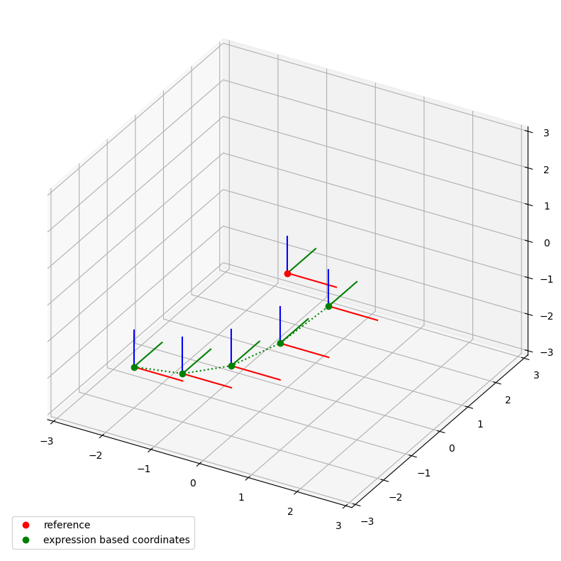
The following systems z-position will change quadratically with time while it moves at a constant speed into the x-direction:

expression = "a*t^2 + b*t + c"
parameters = dict(
    a=Q_([0, 0, 0.2], "mm/s^2"), b=Q_([1, 0, 0], "mm/s"), c=Q_([-2, -2, -2], "mm")
)

me = MathematicalExpression(expression=expression, parameters=parameters)
ts = TimeSeries(me)

lcs_expr = LocalCoordinateSystem(coordinates=ts)

1.9. Transformation of spatial data

Note The things covered in this section are not necessary to work with WelDX and can be skipped. Data transformations can be done much easier using the CoordinateSystemManager class.

The LocalCoordinateSystem only defines how the different coordinate systems are oriented towards each other. If you want to transform spatial data that is defined in one coordinate system (for example specimen geometry/point cloud) you have to use the CoordinateSystemManager, which is discussed in the next tutorial, or do the transformation manually. For the manual transformation, you can get all you need from the LocalCoordinateSystem using its accessor properties:

orientation = lcs_a_in_b.orientation
coordinates = lcs_a_in_b.coordinates

The returned data is an xarray.DataFrame. In case you are not used to work with this data type, you can get a numpy.ndarray by simply using their data property:

orientation_numpy = lcs_a_in_b.orientation.data
coordinates_numpy = lcs_a_in_b.coordinates.data

Keep in mind, that you actually get an array of matrices (orientation) and vectors (coordinates) if the corresponding component is time dependent. The transformation itself is done by the equation:

$$v_b = O_{ab} \cdot v_a + c_{ab}$$

where $v_a$ is a data point defined in coordinate system a, $O_{ab}$ is the orientation matrix of a in b, $c_{ab}$ the coordinates of a in b and $v_b$ the transformed data point.

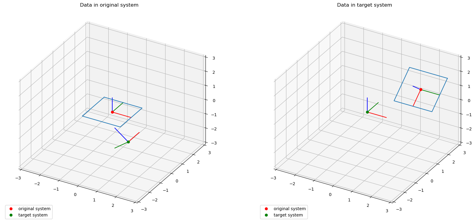
Here is a short example that transforms the points of a square from one coordinate system to another. First we create a set of points with the coordinates meant to be defined in the reference system:

data = np.array(
    [[-1, 1, 0], [1, 1, 0], [1, -1, 0], [-1, -1, 0], [-1, 1, 0]], dtype=float
)

points_in_ref = Q_(data.transpose(), "mm")

Now we create the target system:

lcs_target_in_ref = LocalCoordinateSystem.from_euler(
    sequence="zy", angles=[90, -45], degrees=True, coordinates=Q_([2, -2, 0], "mm")
)

For the transformation from the reference system to the target system we actually need the orientation and coordinates of the inverted target system:

lcs_ref_in_target = lcs_target_in_ref.invert()
t_mat = lcs_ref_in_target.orientation.data
t_vec = lcs_ref_in_target.coordinates.data

Now we use the formula we discussed earlier:

points_in_target = np.matmul(t_mat, points_in_ref) + t_vec[:, np.newaxis]

Note that we needed to broadcast the values of t_vec using [:, np.newaxis] because we are not working with a single point but an array of points. Since we now have the data available in both coordinate systems, we can create the following plots:

1.10. Internal xarray structure

The local coordinate system and many other components of the WelDX package use xarray data frames internally. So it is also possible to pass xarray.DataArrays to a lot of methods. However, they need a certain structure which will be described here. If you are not familiar with the xarray package, you should first read the documentation.

To pass a xarray.DataArray as coordinates to a LocalCoordinateSystem, it must at least have a dimension c. It represents the location in 3d space of the coordinate system and must always be of length 3. Those components must be named coordinates of the data frame (coords={"c": ["x", "y", "z"]}). An optional dimension is time. It can be of arbitrary length, but the timestamps must be added as coordinates.

The same conventions that are used for the coordinates also apply to the orientations. Additionally, they must have another dimension v of length 3, which are enumerated ("v": [0, 1, 2]). c and v are the rows and columns of the orientation matrix.

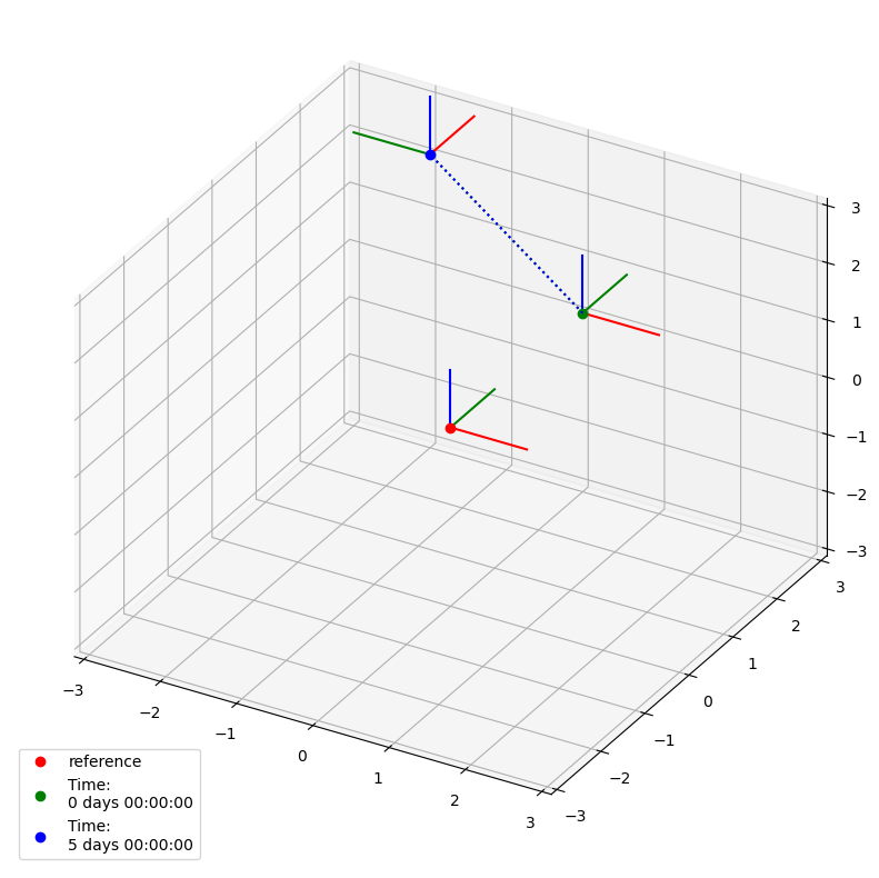
Here is an example. Time dependent coordinates are defined as follows:

time = pd.TimedeltaIndex([0, 5], "D")
coordinates_q = Q_([[0, 3, 0], [-2, 3, 2]], "mm")

coordinates_da = xr.DataArray(
    data=coordinates_q,
    dims=["time", "c"],
    coords={"time": time, "c": ["x", "y", "z"]},
)

/tmp/ipykernel_3435/3776468396.py:1: FutureWarning: The 'unit' keyword in TimedeltaIndex construction is deprecated and will be removed in a future version. Use pd.to_timedelta instead.
  time = pd.TimedeltaIndex([0, 5], "D")

The definition of time dependent orientations is quite similar:

orientation_q = [
    [[1, 0, 0], [0, 1, 0], [0, 0, 1]],
    [[0, -1, 0], [1, 0, 0], [0, 0, 1]],
]

orientation_da = xr.DataArray(
    data=orientation_q,
    dims=["time", "c", "v"],
    coords={"time": time, "c": ["x", "y", "z"], "v": [0, 1, 2]},
)

Now we can create a new LocalCoordinateSystem:

lcs_xr = LocalCoordinateSystem(orientation=orientation_da, coordinates=coordinates_da)

Here is the resulting plot:

The weldx.utility package contains two utility functions to create xarray data frames that can be passed as orientation and coordinates to an LocalCoordinateSystem. They are named xr_3d_vector and xr_3d_matrix. Here are the links to the corresponding API documentation for vectors and matrices.