7. TimeSeries Tutorial

7.1. imports

import numpy as np
import pandas as pd

from weldx import Q_, MathematicalExpression, TimeSeries

7.2. about the TimeSeries class

The TimeSeries class is a general way to describe the behavior of a scalar or multidimensional quantity over time.

In principle, two different approaches can be taken to define this behavior:

1. use a symbolic mathematical expression to exactly define the time dependent relationship

2. provide discrete values with associated times and define how to interpolate the time dependent behavior between timesteps

After creating a TimeSeries we can query the values at any point in time using the TimeSeries.interp_time() method.

7.3. about unit support when using TimeSeries

TimeSeries only works with Quantity objects to enforce consistency in handling unit conversions, that means that all values have to be associated with a unit. When working with dimensionless data, this has to be explicitly stated by providing a dimensionless unit "". The preferred way to create quantity data is to use the weldx-Q_ constructor.

7.4. About time formats

• Currently the time representation only supports relative Timedelta-like time values and no absolute Timestamp information.

• To describe time values, either pandas.TimedeltaIndex or pint.Quantity describing time values are supported as we will show below.

7.5. Discrete Values Examples

7.5.1. simple constant examples

7.5.1.1. scalar constants

We start by creating the simplest TimeSeries object possible: a simple constant (scalar) value. Since constant values are inherently independent of time we only have to provide the value to the TimeSeries. Keep in mind to use Quantities here as well.

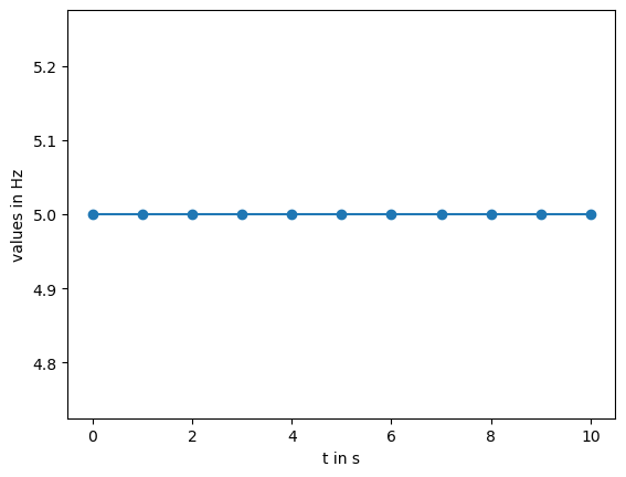
Lets create a simple TimeSeries representing a constant frequency of 5 Hz.

ts_constant = TimeSeries(Q_(5, "Hz"))
print(ts_constant)

<TimeSeries>
Constant value:
	5
Units:
	Hz

Let’s evaluate our constant timeseries at each second over a span of 10 seconds. To do this, we first create a pandas.TimedeltaIndex that represents our desired timespan.

t = pd.timedelta_range(start="0s", end="10s", freq="s")
t

TimedeltaIndex(['0 days 00:00:00', '0 days 00:00:01', '0 days 00:00:02',
                '0 days 00:00:03', '0 days 00:00:04', '0 days 00:00:05',
                '0 days 00:00:06', '0 days 00:00:07', '0 days 00:00:08',
                '0 days 00:00:09', '0 days 00:00:10'],
               dtype='timedelta64[ns]', freq='S')

We can now use these timestamps to evaluate our constant timeseries.

ts_constant.interp_time(time=t)

<TimeSeries>
Time:
	Time:
TimedeltaIndex(['0 days 00:00:00', '0 days 00:00:01', '0 days 00:00:02',
                '0 days 00:00:03', '0 days 00:00:04', '0 days 00:00:05',
                '0 days 00:00:06', '0 days 00:00:07', '0 days 00:00:08',
                '0 days 00:00:09', '0 days 00:00:10'],
               dtype='timedelta64[ns]', freq=None)
Values:
	[5. 5. 5. 5. 5. 5. 5. 5. 5. 5. 5.]
Interpolation:
	step
Units:
	Hz

It is important to note, that TimeSeries.interp_time() will always return its results as an xarray object with the following structure:

• a single named time dimension with the evaluated timestamps as coordinate values

• the data consisting of our constant value as a Quantity

We can also create a simple plot, using the TimeSeries.plot function:

ts_constant.plot(time=t, marker="o")

<Axes: xlabel='t in s', ylabel='values in Hz'>

7.5.1.2. multi-dimensional constant example

We can also create multi-dimensional constant values. For this to work, we have to wrap our value into another dimension of length 1 to indicate a constant time axis. For example, lets represent a single constant cartesian vector with our TimeSeries:

ts_constant_vector = TimeSeries(Q_([[0, 2, 10]], "cm"))
print(ts_constant_vector)

<TimeSeries>
Constant value:
	[ 0  2 10]
Units:
	cm

Interpolation still works as expected:

ts = ts_constant_vector.interp_time(time=t)
print(ts)

<TimeSeries>
Time:
	Time:
TimedeltaIndex(['0 days 00:00:00', '0 days 00:00:01', '0 days 00:00:02',
                '0 days 00:00:03', '0 days 00:00:04', '0 days 00:00:05',
                '0 days 00:00:06', '0 days 00:00:07', '0 days 00:00:08',
                '0 days 00:00:09', '0 days 00:00:10'],
               dtype='timedelta64[ns]', freq=None)
Values:
	[[ 0.  2. 10.]
 [ 0.  2. 10.]
 [ 0.  2. 10.]
 [ 0.  2. 10.]
 [ 0.  2. 10.]
 [ 0.  2. 10.]
 [ 0.  2. 10.]
 [ 0.  2. 10.]
 [ 0.  2. 10.]
 [ 0.  2. 10.]
 [ 0.  2. 10.]]
Interpolation:
	step
Units:
	cm

7.5.2. Interpolation examples

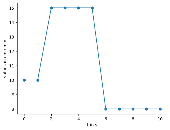
The main idea of TimeSeries is to reflect time dependent data. For values that change over time, we can define discrete values at specific points in time and pass the interpolation method on to the TimeSeries. Let’s say we want a value representing a velocity that starts at 10 cm/min, jumps to 15 cm/min between 2 and 6 seconds of our experiment and stays at 8 cm/min afterwards. To represent this behavior we can use the step interpolation method.

ts_step = TimeSeries(
    data=Q_([10, 15, 8], "cm/min"),
    time=pd.TimedeltaIndex(data=[0, 2, 6], unit="s"),
    interpolation="step",
)
ts_step

<TimeSeries>
Time:
	Time:
TimedeltaIndex(['0 days 00:00:00', '0 days 00:00:02', '0 days 00:00:06'], dtype='timedelta64[ns]', freq=None)
Values:
	[10 15  8]
Interpolation:
	step
Units:
	cm / min

lets interpolate this to our previous timeline and see the results

ts = ts_step.interp_time(t)
print(ts)
ts.plot(marker="o")

<TimeSeries>
Time:
	Time:
TimedeltaIndex(['0 days 00:00:00', '0 days 00:00:01', '0 days 00:00:02',
                '0 days 00:00:03', '0 days 00:00:04', '0 days 00:00:05',
                '0 days 00:00:06', '0 days 00:00:07', '0 days 00:00:08',
                '0 days 00:00:09', '0 days 00:00:10'],
               dtype='timedelta64[ns]', freq=None)
Values:
	[10 10 15 15 15 15  8  8  8  8  8]
Interpolation:
	step
Units:
	cm / min

<Axes: xlabel='t in s', ylabel='values in cm / min'>

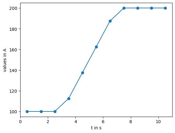
The second supported interpolation style is linear. Let’s use this to create a timeseries that increases from 100 A to 200 A between 3 seconds and 7 seconds of the experiment.

ts_linear = TimeSeries(
    data=Q_([100, 200], "A"),
    time=pd.TimedeltaIndex(data=[3, 7], unit="s"),
    interpolation="linear",
)
ts_linear

<TimeSeries>
Time:
	Time:
TimedeltaIndex(['0 days 00:00:03', '0 days 00:00:07'], dtype='timedelta64[ns]', freq=None)
Values:
	[100 200]
Interpolation:
	linear
Units:
	A

ts = ts_linear.interp_time(t)
print(ts)
ts.plot(marker="o")

<TimeSeries>
Time:
	Time:
TimedeltaIndex(['0 days 00:00:00', '0 days 00:00:01', '0 days 00:00:02',
                '0 days 00:00:03', '0 days 00:00:04', '0 days 00:00:05',
                '0 days 00:00:06', '0 days 00:00:07', '0 days 00:00:08',
                '0 days 00:00:09', '0 days 00:00:10'],
               dtype='timedelta64[ns]', freq=None)
Values:
	[100. 100. 100. 100. 125. 150. 175. 200. 200. 200. 200.]
Interpolation:
	linear
Units:
	A

<Axes: xlabel='t in s', ylabel='values in A'>

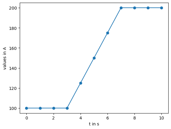
One important note about TimeSeries.interp_time() that can be seen from the plot above: Even though we only defined the TimeSeries discrete values at timesteps 3s and 7s, the interpolation gives back results outside of that timerange as well. This is the current intended behavior of all timeseries interpolations. The last defined values will be propagated as constant values outside of the initial time range. The initial and final values are preserved even when not included in the interpolation time.

ts = ts_linear.interp_time(t + pd.Timedelta(0.5, "s"))
print(ts)
ts.plot(marker="o")

<TimeSeries>
Time:
	Time:
TimedeltaIndex(['0 days 00:00:00.500000', '0 days 00:00:01.500000',
                '0 days 00:00:02.500000', '0 days 00:00:03.500000',
                '0 days 00:00:04.500000', '0 days 00:00:05.500000',
                '0 days 00:00:06.500000', '0 days 00:00:07.500000',
                '0 days 00:00:08.500000', '0 days 00:00:09.500000',
                '0 days 00:00:10.500000'],
               dtype='timedelta64[ns]', freq=None)
Values:
	[100.  100.  100.  112.5 137.5 162.5 187.5 200.  200.  200.  200. ]
Interpolation:
	linear
Units:
	A

<Axes: xlabel='t in s', ylabel='values in A'>

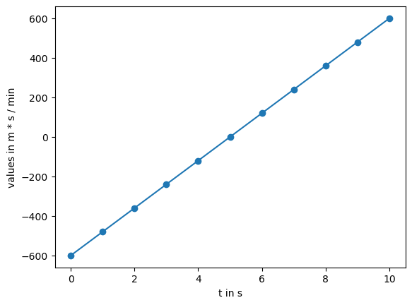
7.6. Mathematical expression examples

The second method to describe our TimeSeries object is by providing a MathematicalExpression that can be evaluated against time parameters.

7.6.1. linear equation example

Let’s create a linear ramp function as an example: $f(t) = a*t + b$.

Note that all parameters must be defined as Quantities in a way that the expression correctly evaluates all dimensions when provided with a time-dimension input (in our case for parameter t)

expr_string = "a*t+b"
parameters = {"a": Q_("120 m/min"), "b": Q_("-10 m")}
expr = MathematicalExpression(expression=expr_string, parameters=parameters)

ts_expr = TimeSeries(data=expr)

ts = ts_expr.interp_time(t)
print(ts)
ts.plot(marker="o")

<TimeSeries>
Time:
	Time:
TimedeltaIndex(['0 days 00:00:00', '0 days 00:00:01', '0 days 00:00:02',
                '0 days 00:00:03', '0 days 00:00:04', '0 days 00:00:05',
                '0 days 00:00:06', '0 days 00:00:07', '0 days 00:00:08',
                '0 days 00:00:09', '0 days 00:00:10'],
               dtype='timedelta64[ns]', freq=None)
Values:
	[-600. -480. -360. -240. -120.    0.  120.  240.  360.  480.  600.]
Interpolation:
	step
Units:
	m * s / min

<Axes: xlabel='t in s', ylabel='values in m * s / min'>

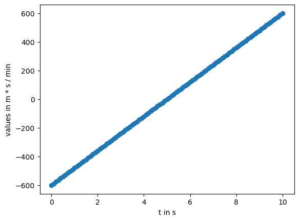
We can also use Quantites with the appropriate dimension as Inputs for our interpolation:

t2 = Q_(np.arange(101) * 100, "ms")
ts = ts_expr.interp_time(t2)
ts.plot(marker="o")

<Axes: xlabel='t in s', ylabel='values in m * s / min'>

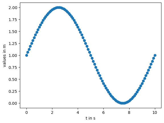
7.6.2. sine example

Of course we can also have more complex examples. Lets create a sine wave function that oscillates around 1 m at a frequency of 36 deg/s.

expr_string = "a*sin(o*t)+b"
parameters = {"a": Q_("1 m"), "b": Q_("1 m"), "o": Q_("36 deg/s")}
expr = MathematicalExpression(expression=expr_string, parameters=parameters)

ts_sine = TimeSeries(data=expr)

ts = ts_sine.interp_time(pd.timedelta_range(start="0s", end="10s", freq="100ms"))
ts.plot(marker="o")

<Axes: xlabel='t in s', ylabel='values in m'>

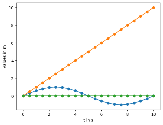
7.6.3. vector example

With careful syntax it is also possible to create multidimensional TimeSeries objects from math expressions.

expr_string = "a*sin(o*t)+b*t"
parameters = {
    "a": Q_(np.asarray([1, 0, 0]), "m"),
    "b": Q_([0, 1, 0], "m/s"),
    "o": Q_("36 deg/s"),
}
expr = MathematicalExpression(expression=expr_string, parameters=parameters)

ts_vector = TimeSeries(data=expr)

ts = ts_vector.interp_time(pd.timedelta_range(start="0s", end="10s", freq="500ms"))
print(ts)

<TimeSeries>
Time:
	Time:
TimedeltaIndex([       '0 days 00:00:00', '0 days 00:00:00.500000',
                       '0 days 00:00:01', '0 days 00:00:01.500000',
                       '0 days 00:00:02', '0 days 00:00:02.500000',
                       '0 days 00:00:03', '0 days 00:00:03.500000',
                       '0 days 00:00:04', '0 days 00:00:04.500000',
                       '0 days 00:00:05', '0 days 00:00:05.500000',
                       '0 days 00:00:06', '0 days 00:00:06.500000',
                       '0 days 00:00:07', '0 days 00:00:07.500000',
                       '0 days 00:00:08', '0 days 00:00:08.500000',
                       '0 days 00:00:09', '0 days 00:00:09.500000',
                       '0 days 00:00:10'],
               dtype='timedelta64[ns]', freq=None)
Values:
	[[ 0.00000000e+00  0.00000000e+00  0.00000000e+00]
 [ 3.09016994e-01  5.00000000e-01  0.00000000e+00]
 [ 5.87785252e-01  1.00000000e+00  0.00000000e+00]
 [ 8.09016994e-01  1.50000000e+00  0.00000000e+00]
 [ 9.51056516e-01  2.00000000e+00  0.00000000e+00]
 [ 1.00000000e+00  2.50000000e+00  0.00000000e+00]
 [ 9.51056516e-01  3.00000000e+00  0.00000000e+00]
 [ 8.09016994e-01  3.50000000e+00  0.00000000e+00]
 [ 5.87785252e-01  4.00000000e+00  0.00000000e+00]
 [ 3.09016994e-01  4.50000000e+00  0.00000000e+00]
 [ 1.22464680e-16  5.00000000e+00  0.00000000e+00]
 [-3.09016994e-01  5.50000000e+00  0.00000000e+00]
 [-5.87785252e-01  6.00000000e+00  0.00000000e+00]
 [-8.09016994e-01  6.50000000e+00  0.00000000e+00]
 [-9.51056516e-01  7.00000000e+00  0.00000000e+00]
 [-1.00000000e+00  7.50000000e+00  0.00000000e+00]
 [-9.51056516e-01  8.00000000e+00  0.00000000e+00]
 [-8.09016994e-01  8.50000000e+00  0.00000000e+00]
 [-5.87785252e-01  9.00000000e+00  0.00000000e+00]
 [-3.09016994e-01  9.50000000e+00  0.00000000e+00]
 [-2.44929360e-16  1.00000000e+01  0.00000000e+00]]
Interpolation:
	step
Units:
	m

Here is a plot showing the x,y,z coordinates:

ts.plot(marker="o")

<Axes: xlabel='t in s', ylabel='values in m'>