2. Time dependent data / Welding current and voltage#
<< PREVIOUS TUTORIAL | NEXT TUTORIAL >>
2.1. Overview#
This tutorial covers:
Accessing and visualizing time dependent data stored inside a
TimeSeriesclass
Requirements:
Opening and navigating through WelDX files (tutorial)
# download the example file for this tutorial

from util import download_tutorial_input_file

download_tutorial_input_file(print_status=False)
2.2. Plotting data#
Two important quantities in welding applications are the welding current and welding voltage. Both are constantly monitored during an experiment. The obtained data is a one dimensional array with time being its only dimension. We will extract both from the file and see what we can do with it. First we read the file and get an overview over its content as we learned in the previous tutorial:
from weldx import WeldxFile

wxfile = WeldxFile("single_pass_weld.wx")
/home/docs/checkouts/readthedocs.org/user_builds/weldx/conda/latest/lib/python3.10/site-packages/asdf/asdf.py:340: AsdfWarning: File 'file:///home/docs/checkouts/readthedocs.org/user_builds/weldx/checkouts/latest/doc/src/tutorials/single_pass_weld.wx' was created with extension URI 'asdf://weldx.bam.de/weldx/extensions/weldx-0.1.1' (from package weldx==0.6.0), which is not currently installed
  warnings.warn(msg, AsdfWarning)
wxfile.info()
root (dict)
├─TCP (LocalCoordinateSystem)
├─coordinate_systems (CoordinateSystemManager)
├─equipment (list)
│ ├─[0] (MeasurementEquipment)
│ ├─[1] (MeasurementEquipment)
│ └─[2] (MeasurementEquipment)
├─measurements (list)
│ ├─[0] (Measurement)
│ ├─[1] (Measurement)
│ ├─[2] (Measurement)
│ └─[3] (Measurement)
├─process (dict)
│ ├─shielding_gas (ShieldingGasForProcedure)
│ ├─weld_speed (TimeSeries)
│ ├─welding_process (GmawProcess)
│ └─welding_wire (dict)
│   ├─class (str)
│   ├─diameter (Quantity)
│   └─wx_user (dict)
│     ├─charge id (str)
│     └─manufacturer (str)
├─reference_timestamp (Timestamp)
├─welding_current (TimeSeries)
├─welding_voltage (TimeSeries)
├─workpiece (dict)
│ ├─base_metal (dict)
│ │ ├─common_name (str)
│ │ └─standard (str)
│ └─geometry (dict)
│   ├─groove_shape (VGroove)
│   └─seam_length (Quantity)
└─wx_user (dict)
  ├─WID (int)
  ├─operator (str)
  └─project (str)
As we can see in the list, there are the top level items welding_current and welding_voltage.
Let’s have a look at the welding current first:
current = wxfile["welding_current"]
The object we extracted is of type TimeSeries as can be seen in the info output.
This is a special type provided by WelDX to deal with time dependent data.
To see a plot of the TimeSeries simply call the built-in .plot() function.
If you are already familiar with matplotlib it is also easy to generate your own plots. We show how to access the underlying data later in this tutorial.
current.plot()
<Axes: xlabel='t in s', ylabel='values in A'>
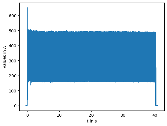
The plot method is an easy and convenient way to quickly visualize a TimeSeries.
It labels the axes automatically and attaches the corresponding units to them.
Depending on the Python environment you are using, there are some things to consider.
Since the plot method uses matplotlib internally, you have to call the matplotlib.pyplot.show function manually after using plot when running a regular Python script file.
Otherwise, the plot won’t show up.
This is not the case if you work with a jupyter notebook, where the plots are generated after each cell execution.
However, while a regular script will open an interactive window for each plot, the plots inside a notebook can’t be modified without additional commands.
To enable interactive matplotlib plots inside a jupyter notebook, uncomment and run the following magic command:
# %matplotlib widget
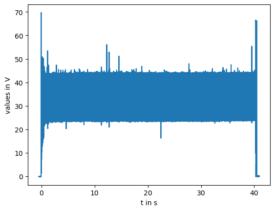
Now let’s plot the welding voltage. Try to interact with the plot if you are running this tutorial as a jupyter notebook.
voltage = wxfile["welding_voltage"]
voltage.plot()
<Axes: xlabel='t in s', ylabel='values in V'>
2.3. Accessing the data#
Now that we know how to get a quick overview over the data by visualizing it with the plot method, let’s have a look on what else we can do with a TimeSeries.
While any number of dimensions in addition to time are supported, we expect the welding current to have no further dimensions.
We can easily check this using the shape property:
current.shape
(414091,)
From the returned value we see that the data indeed only consists of a single dimension. Furthermore, we get the exact number of data points that are stored in the time series.
We already saw in the axes labeling of the plots, that the TimeSeries also stores the units of the data
We can get it by calling the units property:
current.units
As one might expect, the unit of the current is amperes, but it might also have been stored in milliamperes.
Now, if we want to actually access the stored data, we can extract it from the TimeSeries by using its data property.
The returned object is a pint.Quantity.
type(current.data)
pint.Quantity
A pint.Quantity is a thin wrapper around a multi-dimensional array that attaches units to the contained data.
They can be used like NumPy arrays and support most of NumPy’s functions.
For further information on how to work with quantities, consult Pint’s documentation.
An alternative to the data property is the data_array property.
This returns the data as xarray.DataArray:
type(current.data_array)
xarray.core.dataarray.DataArray
Xarray is a powerful tool that makes working with multi-dimensional arrays easier.
When performing operations on an xarray.DataArray, it automatically figures out which dimensions of the operands are compatible with each other and how they need to be combined.
Visit the xarray documentation to learn how to work with xarray classes.
We recommend using either xarray or pint when working with the data, but if you feel more comfortable using NumPy, you can convert both types easily to a numpy.ndarray.
For pint use .magnitude or the short version .m:
type(current.data.magnitude)
numpy.ndarray
For xarray use .data to get the data as pint.Quantity and then .magnitude or .m to receive a numpy.ndarray:
type(current.data_array.data.magnitude)
numpy.ndarray
2.4. Data processing examples#
Before we conclude this lesson, we will show you some simple examples on how to process the data obtained from a weldx file. Pint and Xarray both offer you some basic functions to get the minimal and maximal values of a dataset or to calculate its mean value. Here are the examples for Pint:
current.data.min()
current.data.max()
current.data.mean()
If you exchange .data with .data_array, you will get the same results just as xarray.DataArray.
To demonstrate you some features of Xarray and Pint, we will now do a more involved computation by calculating the electric power using the equation:
$$ P = \frac{1}{T} \int_{t=0}^{T} u \cdot i ;\mathrm{d} t$$
$u$ is the time dependent current, $i$ the time dependent voltage, $t$ the time and $T$ the duration of the measurement.
We will do this step by step to keep it simple and to discuss all the things that need to be considered.
First we will calculate the integral with Xarrays .integrate function which uses the trapezoidal rule.
integral = (voltage.data_array * current.data_array).integrate(
    "time", datetime_unit="s"
)
integral
<xarray.DataArray ()> Size: 8B
<Quantity(486682.2425141883, 'volt * ampere')>
The parameter datetime_unit specifies the unit of the time coordinates during the integration.
Unfortunately, at the time of writing of this tutorial, the unit support of Xarray is still work in progress and not fully implemented.
The result’s unit is just $\mathrm{A \cdot V}$ while it should have been $\mathrm{A \cdot V \cdot s}$.
We correct this by turning the resulting xarray.DataArray into a pint.Quantity (see previous section) and simply multiplying the missing unit.
Therefore we need to import the unit object U_ from weldx.
from weldx import U_

q_integral = integral.data * U_("s")
What remains now is to divide the result by the process duration.
We can get the time data either from the voltage or the current data as they were both measured simultaneously.
It can be accessed with .time which returns a weldx.Time instance.
We will talk a bit more about this class in another tutorial.
For now it is sufficient to know, that it provides a .duration method to get the duration of the contained time data as a new weldx.Time instance and that we can turn it into a quantity using .as_quantity.
So let’s finally calculate the electrical power:
e_power = q_integral / voltage.time.duration.as_quantity()
e_power
We can further simplify this by convert the units manually to Watt with .to or .ito.
The first method creates a new quantity, while the latter one modifies the existing one.
e_power.ito("W")
e_power
If you prefer compact numbers, you can use .to_compact:
e_power.to_compact()
/tmp/ipykernel_3179/1330626161.py:1: UndefinedBehavior: to_compact applied to non numerical types has an undefined behavior.
  e_power.to_compact()
2.5. Conclusion#
This concludes the tutorial about accessing and plotting time dependent data.
We have learned about some basic functionalities of the TimeSeries class and know now, how to get the data for further processing and how to quickly visualize it, using the plot method.